



The frustrating part of SEO experimentation that nobody really warns you about: the change you shipped in March might not show its full effect until June, and by June your traffic is also getting pushed around by seasonality, a core update, a competitor's redesign, and the fact that your sales team ran a promo that flooded the site with links.
So you look at your dashboard, see traffic up 14%, and you have absolutely no honest way to say how much of that was your change.
This is the whole problem with lagged SEO experiment measurement. Ranking effects don't land on deploy day. They diffuse over weeks. And the longer the lag, the more contaminating noise piles into your measurement window. Most teams either declare victory too early, or give up and call it "directionally positive" — which is a polite way of saying "we have no idea."
This post covers the statistical plumbing that actually lets you answer the question. Synthetic controls, cohort alignment, seasonality decomposition, and how to set a confidence window you can defend in a meeting. There's SQL you can steal and a template for minimum detectable effect (MDE) so you stop running experiments that were never going to be readable in the first place.
The core mistake: measuring on calendar time instead of exposure time
Almost every broken long-lag readout comes from the same root error. Teams align their analysis to the deploy date instead of the exposure date for each URL.
Say you're rolling out a template change to 4,000 product pages. Google doesn't recrawl and reprocess all 4,000 on day one. Some get picked up in 3 days, some in 3 weeks, a long tail sits untouched for two months. If you draw a vertical line at the deploy date and compare "before vs after," you're averaging pages that have been fully re-evaluated against pages Google hasn't even looked at yet. Your effect gets smeared into mush.
The fix is building the analysis around cohort alignment: each URL gets a "day 0" defined by when it was actually recrawled after the change, not when you pushed the code. You pull that recrawl timestamp from your log files, then measure each URL's performance relative to its own exposure clock.
This one shift — calendar time to exposure time — usually recovers a signal that looked like noise. A change that reads as "+2%, not significant" on calendar alignment can turn into "+9% within 21 days of recrawl, tight interval" once you align on exposure. Same data. The measurement was just wrong.
A quick SQL pattern for exposure-aligned cohorts
WITH cohort AS ( SELECT g.url, g.date, g.clicks, g.impressions, g.position, DATEDIFF(g.date, r.firstrecrawlafterdeploy, DAY) AS dayssinceexposure FROM gscdaily g JOIN urlrecrawl r USING (url) ) SELECT dayssinceexposure, COUNT(DISTINCT url) AS urls, SUM(clicks) AS clicks, SAFEDIVIDE(SUM(clicks), SUM(impressions)) AS ctr, AVG(position) AS avgposition FROM cohort WHERE dayssinceexposure BETWEEN -28 AND 56 GROUP BY dayssinceexposure ORDER BY dayssinceexposure;
Now dayssinceexposure = 0 means the same operational moment for every URL, regardless of when it actually deployed. Negative days are your pre-period baseline. This alone makes the rest of the analysis honest.
Synthetic control: building the counterfactual you actually need
The hardest thing to prove in SEO is the counterfactual — what your treated pages would have done if you'd changed nothing. Holdouts help, but on long-lag tests your holdout group drifts too. It gets hit by the same core update, rides the same seasonal curve. A raw treated-vs-holdout diff is better than nothing but still leaks.
Stop losing visibility in search results.
GoSeofy helps you monitor, analyze, and improve your SEO performance with ease.
- Comprehensive keyword tracking
- Backlink quality monitoring
- Real-time SEO performance reports
No credit card required
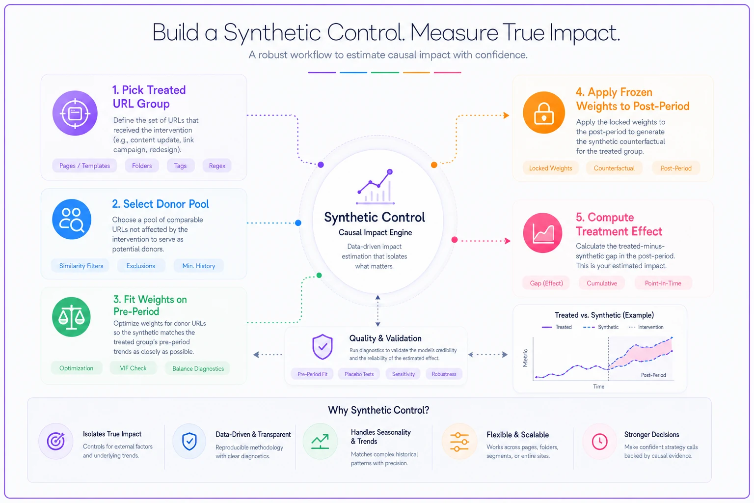
Synthetic control fixes this by building a fake version of your treated group out of a weighted blend of untreated pages that historically tracked it closely. Instead of "here's a holdout group we hope is comparable," you're saying "here's a combination of pages that matched the treated group's behavior for six months before the change, so their post-change path is a defensible stand-in for the counterfactual."
The workflow, in plain terms:
-
Pick your treated URL group and a large donor pool of untreated URLs that never received the change.
-
Use the pre-period (say 12–16 weeks before exposure) to fit weights on donor pages so their weighted sum reproduces the treated group's clicks/position curve as closely as possible.
-
Apply those frozen weights to the post-period. The weighted donor curve is your synthetic control.
-
The gap between the actual treated line and the synthetic line, after exposure day 0, is your estimated effect.
The insight most people miss: your donor pool has to be genuinely untreated and genuinely comparable in intent. Sneak transactional pages into the donor set for an informational-page test and the seasonality patterns won't match — your synthetic control fits garbage. Segment your donor pool by intent tier and page type first. The pre-period fit quality (how tightly the synthetic tracks the real line before day 0) is your honesty check. If it can't reproduce history, don't trust its counterfactual.
Segment your donor pool by intent tier and page type before fitting weights to avoid mismatched seasonal patterns.
Here's the workflow visualized.
The pre-period fit quality (how tightly the synthetic tracks the real line before day 0) is your honesty check. If it can't reproduce history, don't trust its counterfactual.
Seasonality decomposition, because "up 14%" might just be November
Long-lag windows almost always straddle a seasonal shift. Home services climb into spring. Retail bends around Q4. B2B dips in August and over the holidays. If your measurement window is eight weeks, you can easily attribute a seasonal tailwind to your experiment — and just as easily miss a real effect because a headwind ate it.
Decomposition splits an observed series into three parts: trend, seasonal, and residual. You care about the residual — that's what's left after you strip the predictable stuff, and it's where your experiment's effect actually lives.
You don't need anything fancy. A classic multiplicative decomposition using a trailing 52-week seasonal index works fine for most sites:
-- weekly seasonal index from a full prior year, per page-type WITH weekly AS ( SELECT pagetype, EXTRACT(WEEK FROM date) AS wk, SUM(clicks) AS clicks FROM gscdaily WHERE date BETWEEN DATESUB(CURRENTDATE(), INTERVAL 104 WEEK) AND DATESUB(CURRENTDATE(), INTERVAL 52 WEEK) GROUP BY pagetype, wk ), avgwk AS ( SELECT pagetype, AVG(clicks) AS meanclicks FROM weekly GROUP BY pagetype ) SELECT w.pagetype, w.wk, w.clicks / a.meanclicks AS seasonalindex FROM weekly w JOIN avgwk a USING (pagetype);
Then divide your current weekly clicks by that page-type's seasonal index before comparing treated vs synthetic. A subtle mistake here: people compute one global seasonal curve for the whole site. But a blog cluster and a product catalog have completely different seasonal shapes. Decompose per page type, or you'll deseasonalize one segment using another's rhythm.
Worth naming explicitly: if you only deseasonalize and skip the synthetic control, you've handled seasonality but not core updates or competitor moves. If you only build a synthetic control, you've handled broad market drift but seasonal noise still inflates your confidence interval. You want both. They cover different failure modes.
Minimum detectable effect: decide if the test is even readable before you run it
This is the step that saves the most wasted quarters. Before launching a long-lag experiment, calculate the smallest effect your setup could actually detect given your traffic and noise levels. If your MDE is 12% and your change realistically moves things 4%, the experiment is unreadable by design — you'll get an inconclusive result no matter what happens, and you'll have burned three months finding that out.
| Factor | Effect on MDE | Practical note |
|---|---|---|
| Sample size (URLs + clicks) | More → smaller MDE | Thin pages inflate variance badly |
| Residual variance after decomposition | Lower → smaller MDE | Deseasonalizing shrinks this a lot |
| Length of measurement window | Longer → smaller MDE, but more contamination | Trade-off, not a free lunch |
| Quality of synthetic pre-fit | Better fit → smaller MDE | Poor donors = wide intervals |
A rough operational template to gut-check readability:
-
Pull the pre-period residual standard deviation of weekly clicks for the treated group (after deseasonalizing).
-
Compute the standard error of your treated-minus-synthetic gap across the pre-period weeks.
-
MDE ≈ 2.8 × that standard error (roughly the 80% power, 95% confidence rule of thumb for a two-sided test).
-
Compare MDE to the effect size you actually expect from this change.
-
If expected effect < MDE, either expand the cohort, extend the window, or don't run it as a formally measured experiment — ship it as a bet instead.
That last option is genuinely underrated. Not every change needs to be a formally measured experiment. Some are just good ideas you deploy without pretending you'll read them. Knowing which is which is most of the skill.
Setting a confidence window you can actually defend
A confidence window in a long-lag context has two dimensions people tend to conflate: the statistical interval (how uncertain the effect estimate is) and the temporal window (which days after exposure you're actually counting as "the effect").
For the temporal window, don't pick it after seeing the data — that's how people accidentally p-hack their way to a win. Set it upfront based on how the effect physically propagates. A typical readable window looks like:
-
Days -28 to -1 pre-period baseline for synthetic fitting.
-
Days 0 to 13 early diffusion, usually noisy, don't over-read.
-
Days 14 to 42 the primary measurement window for most template/content changes.
-
Days 43+ stabilization check — is the effect holding or decaying?
For the statistical interval, bootstrap it. Resample your donor weights and recompute the treated-minus-synthetic gap a few thousand times, then take the 2.5th and 97.5th percentiles of the effect distribution. This gives you an interval that honestly reflects donor-pool uncertainty, which a naive t-test never will.
The mistake to avoid: reporting a point estimate with no window at all. "+8%" is nearly meaningless. "+8%, 95% interval of +3% to +13%, measured days 14–42 post-recrawl, synthetic pre-fit R² of 0.94" is something you can put a budget decision behind.
A real scenario: a mid-size home-services site
A regional HVAC and plumbing company with roughly 900 location-and-service landing pages rewrote its service-page template — new intro structure, FAQ schema, tighter internal links. Classic long-lag change. Their first readout, done on calendar alignment, showed organic clicks up around 11% and the team was ready to call it a win.
The problem: they deployed in late February, and spring is exactly when HVAC search demand climbs. Their control-free, calendar-aligned "+11%" was mostly the season.
Reworking it properly — aligning each page to its actual recrawl date from server logs, building a synthetic control from roughly 300 untouched pages in comparable metros, and deseasonalizing using the prior year's spring index for service pages specifically — the honest effect came out closer to +4% to +6%, with a 95% interval that barely cleared zero on the low end. Real, but a third the size of the headline number.
That downgrade sounds like bad news. It wasn't. It stopped them from rolling the template to their entire catalog under a false 11% assumption, and it set a realistic baseline so the next iteration could be measured against something true. A follow-up tweak a quarter later added a few more points that they could actually trust.
When this level of rigor makes sense — and when it doesn't
Not every SEO change warrants the full statistical treatment. Part of getting good at this is knowing when to apply it and when to just ship.
Do this when:
-
The change touches enough URLs and clicks to be statistically readable (run the MDE check first).
-
The measurement window will straddle a seasonal shift or a likely core update.
-
The decision downstream is expensive — a full-catalog rollout, a big content investment, killing a strategy.
Skip the full machinery when:
-
The change is tiny, cheap, and reversible. Just ship it.
-
Traffic is so low that MDE is hopeless regardless — no amount of statistics rescues 40 clicks a week.
-
You need a decision this week. Long-lag rigor is for long-lag questions.
Who should not attempt this yet: teams whose GSC and log data don't reconcile. If your recrawl timestamps and performance data live in separate, untrusted silos, exposure alignment will produce confident nonsense. Fix the data foundation before the statistics — this is exactly the kind of thing that benefits from a well-built SEO data pipeline for revenue attribution where your log, GSC, and conversion tables actually join cleanly.
Making this repeatable instead of a one-off heroic analysis
The teams that get good at this don't rebuild the whole thing per experiment. They standardize the recipe: a cohort-alignment view, a donor-pool builder segmented by intent and page type, a per-segment seasonal index that refreshes weekly, and a bootstrap function that spits out the effect interval and pre-fit quality automatically. Then every experiment readout runs through the same query pattern with different inputs.
That standardization is what turns experimentation from an occasional science project into an operating cadence — and it pairs naturally with a broader enterprise SEO experimentation program where results feed a shared ledger instead of dying in someone's private spreadsheet.
The honest value of getting lagged experiments right is partly defensive: knowing when you can't read a result keeps you from betting the catalog on seasonal noise dressed up as a win. Align on exposure, build a real counterfactual, strip out the season, and set your window before you look. Do that consistently and your readouts stop being arguments and start being decisions.
Align on exposure, build a real counterfactual, strip out the season, and set your window before you look.
Do that consistently and your readouts stop being arguments and start being decisions.
Ready to elevate your search rankings?
Join 5,000+ businesses using GoSeofy to increase organic traffic, optimize content, and outperform competitors online.